Date Functions:

Let`s now check some important Excel date functions such as TODAY, NOW, YEAR, MONTH, DATE and EDATE.

Date Function TODAY:

Every date in Excel is associated with a specific number. The number 1 represents the date of 1st of January 1900. Number 2 is then associated with the day after (2nd January 1900), and this sequence goes on and on.

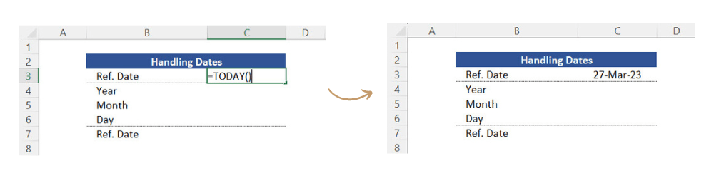
Based on that, the first date function you need to understand is the function TODAY which basically displays the “specific number” associated with your current date. As that information comes directly from your computer calendar, this function does not require any arguments. Follow the steps below on the spreadsheet you downloaded:

1. Insert the function TODAY in cell C3.

2. You can then simply close brackets and press ENTER. Today`s date will show up on your screen.

Date Function NOW:

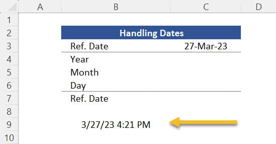
If in addition to the date you also need the exact time you are at, you can then use the function NOW. This is one of the date functions which does not require any arguments as it`s connected to your computer calendar and clock. Follow the steps below:

1. So, select any cell of your sheet and insert the function NOW.

2. As this function also does not require any arguments, simply close brackets and press ENTER.

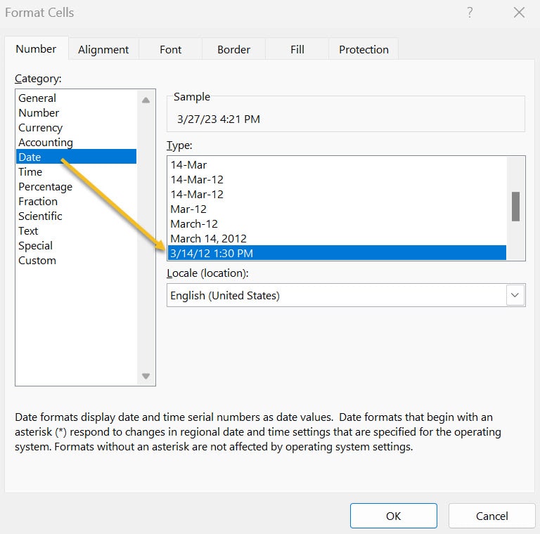
3. Make sure you have the correct format set for that cell, which shows both date and time.

4. Your current date and time will be shown in the cell you chose.

Calendar Functions (YEAR, MONTH, DAY)

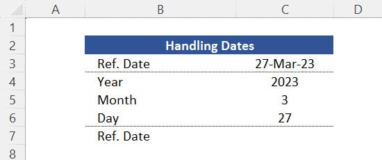
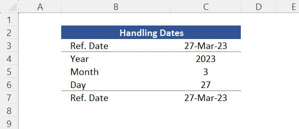
The calendar functions YEAR, MONTH and DAY are used to extract their respective information from whatever date you have in your spreadsheet. Using the date you inserted in cell C3 as a reference point, follow the steps below:

1. So, insert the function YEAR in cell C4. The argument “Serial Number” is basically the date from cell C3. The year will be extracted from that date.

2. Next, you need to insert the function MONTH in cell C5. Again, the argument “Serial Number” will be the date from cell C3. A number from 1 to 12 will be extracted for you which basically represents the number of the month you are in.

3. Finally, insert the function DAY in cell C6. Use cell C3 as the argument of this function as well. The specific day of the month will be extracted for you.

These functions in isolation can be quite handy for a variety of uses in your spreadsheets:

• Function YEAR: When you isolate the “year” of a date, you can easily use that information to calculate periodic events in a forecast calculation of your business (e.g. overhaul maintenance of assets taking place every 2 or 3 years for example).
• Function MONTH: In isolation, the “month” of a date can help you to perform a calculation regarding tax assessment in a financial model (e.g. Tax to be calculated only in the months of March (Month 3) or April (Month 4)).
• Function Day: In isolation, the variable “day” can be used to calculate your staff payment for example (e.g. payments taking place on the 5^th of every month).

Date Function DATE:

This is one of the most important date functions as it directly works with the calendar functions. If you now need to work the other way around (i.e. creating a date with the isolated parameters “Year”, “Month” and “Day”), you can simply use the date function DATE. Follow the steps below:

1. So, insert the function DATE in cell C7

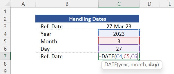
2. Then use cell C4 as the argument “year”

3. After that, use cell C5 as the argument “month”

4. Next, use cell C6 as the argument “day”

5. Finally, close brackets and press ENTER. Now cell C6 will show the same initial date you had in cell C3.

Using Calendar Functions to calculate paste and future dates in Excel:

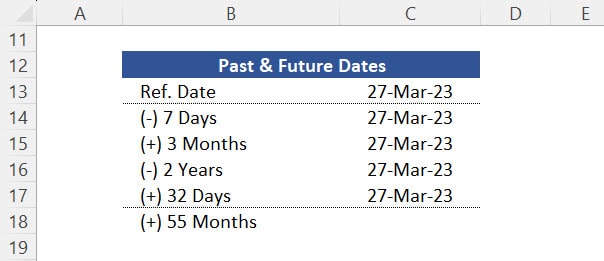
When you have a clear understanding of calendar functions and how to combine them, it becomes very easy to calculate past and future dates in Excel. So before you carry on, copy cell C7 and paste that date (as values) in cell C13. This will be our reference point going forward. You can then combine the calendar functions to calculate alternative dates as per image below:

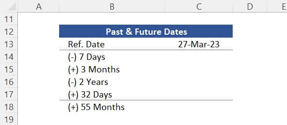
For a task like this, the first thing you need is to create a combined calendar function which you can replicate in the range C14 to C17.

Creating a Template:

Follow the steps below:

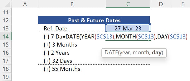
1. So, insert the function DATE in cell C14.

2. For the argument “year”, use the function YEAR. The argument “serial number” of this function YEAR must be cell C13. Close brackets to complete this sub function and press comma to skip to the next argument.

3. After that, for the argument “month”, use the function MONTH. The argument “serial number” of this function MONTH must be cell C13 again. Close brackets to complete this sub function and press comma to skip to the last argument.

4. For the argument “day”, use the function DAY. The argument “serial number” of this function DAY must be one more time cell C13. Close brackets once to complete this sub function and close brackets again to complete the main function DATE.

5. After that, insert “absolute reference” in all the arguments of this function by pressing F4 in those arguments.

6. At last, expand the function you created in cell C14 all the way to cell C17.

Calculating the alternative dates:

To identify alternatives dates simply follow the steps below:

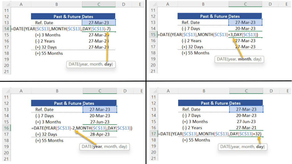
a. 7 Days ago: Subtract 7 from the argument “day” of the function DATE you built in cell C14.

b. 3 Months from now: Add 3 to the argument “month” of the function DATE you built in cell C15.

c. 2 Years ago: Subtract 2 from argument “year” of the function DATE you built in cell C16.

d. 32 days from now: Add 32 to the argument “day” of the function DATE you built in cell C17.

Date Function EDATE:

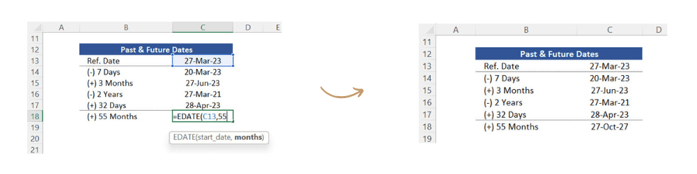
You constantly need to work with alternative dates based on different number of “months”, you can also use the date function EDATE. You can test that function in cell C18 where you need to calculate a date which is 55 months over the reference date from cell C13. Follow the steps below:

1. So, insert the function EDATE in cell C18.

2. After that, the argument “start date” is again cell C13.

3. The argument “months” is basically the number of months you need which in this case is 55. So type that number, close brackets and press ENTER. The correct date will show up in the screen.