Countdown Calendar & Function NETWORKDAYS

Let`s now learn how to build a Countdown Calendar in Excel. Further down we will also cover the important function NETWORKDAYS.

Building a Countdown Calendar

An interesting use of the Excel function TODAY is when you need to create a Countdown Calendar which is very useful whenever you need to manage corporate events, sales targets, and projects in general in a spreadsheet.

In the example below, let`s assume you are investing in a property development project.

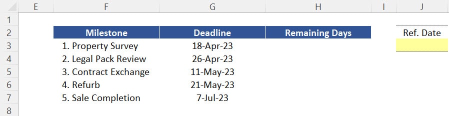
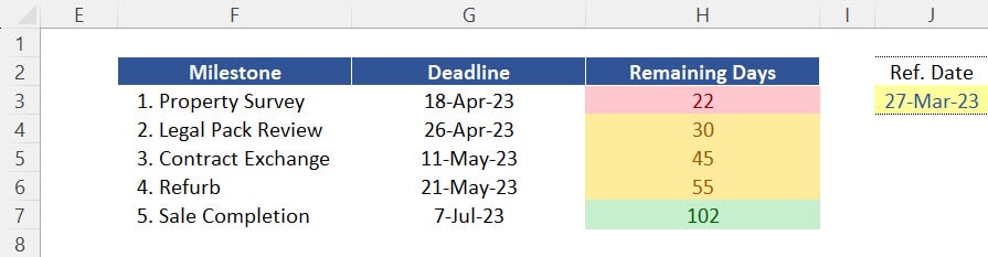
In this project we have 5 defined milestones (column F). For each of those milestone we can see a specific deadline to achieve (column G). We now need to identify how many days are left for the deadlines of each of those milestones. We must perform these calculations in column H. The reference point for the calculation is “today`s date” which we need to calculate in cell J3 through the Excel function TODAY.

Countdown Calendar – Calculation

To calculate the variable “Remaining Days”, follow the steps below:

1. Insert the function TODAY in cell J3. As we saw in Part I of this tutorial, this function does not require any arguments as it`s basically linked to your computer calendar. So, close brackets and press ENTER.

2. In cell H3, press equals (“=”) and subtract cell J3 from cell G3. As we need to use the same reference point across the entire range H3:H7, insert “absolute reference” in cell G3 by pressing the shortcut “F4” over it and then pressing CTRL + ENTER.

3. Now select the entire range H3:H7 and press F2 and then CTRL + ENTER to expand the initial formula across the entire range.

We just completed the backbone of the Countdown Calendar. Now anytime you open your Excel file, the function TODAY will be updated and therefore the variable “Remaining Days” will decrease by 1 day whenever 1 day is passed. However, we now need to make it look more professional and dynamic, which can be done through 2 simple adjustments: (a) Eliminating negative numbers and (b) Applying Conditional Formatting.

Countdown Calendar Adjustment 1: Eliminating negative numbers

The first adjustment is straight forward. As the number of “Remaining Days” decreases every day the file is updated, at some point that deadline will be overlapped and as a result negative numbers will start to show up in your file which basically means that the specific deadline you are assessing is now expired. To correct that, follow the 2 steps below:

Step 1: Function MAX

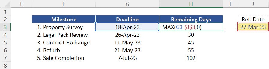
1. Press F2 in cell H3 which is currently showing the difference between cells G3 and J3. Here we need to force this difference to be always positive.

2. To do that, insert the function MAX just after the equals sign and press TAB to accept that function. The first argument of the function is the difference itself so press comma to skip to the second argument. Here simply type the number 0. By doing this the result of this function will always be the maximum between the difference of dates and 0 and therefore a positive value will always be returned by this function. You can then close brackets and press ENTER.

Step 2: Function IF

1. Now, press F2 to edit that cell. Select the entire function MAX and copy it (CTRL + C).

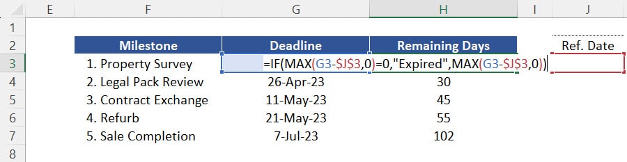
2. Just after the equals sign, insert the conditional function IF and press TAB to accept it. We can then work on the logical test of this function which is “MAX (G3 – $J$3) = 0”. For the “Value if True” argument, type the word “Expired”. For the “Value if False” argument, simply press CTRL + V to paste the function MAX you copied on step 3 above. By taking this approach the result of your calculation will either be a positive number, which demonstrates how many days we have to achieve each deadline, or the word “Expired” otherwise.

3. Expand the same combined function to the entire range H3:H7.

Countdown Calendar Adjustment 2: Applying Conditional Formatting

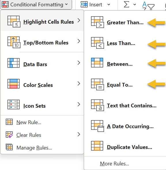
The second adjustment in your Countdown Calendar is also simple where a specific colour needs to be highlighted for each possibility of result displayed in the variable “Remaining Days”. This can be done through the tool “Conditional Formatting”. In this example we can highlight the cells we want based on 4 rules: (a) “Greater Than” (b) “Less Than” (c) “Between”,  and (d) “Equal To”.

Inserting the Conditional Formatting Rules:

To apply conditional formatting to your range, follow the steps below:

1. Select the range H3:H7 and go to the conditional formatting menu and choose the option “Highlight Cells Rules”.

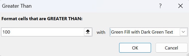
2. Choose the first option “Greater Than”. Here let’s for example insert the number 100 as our threshold and let’s select the color green for the background. Therefore, anytime the variable “Remaining Days” is greater than 100 days, a green background color will be highlighted in any cell of that range. Click on OK to accept that rule.

3. Next, go back to the Conditional Formatting menu and this time select the rule “Less Than”. This time, let`s insert the number 30 as a threshold and let’s keep the default red color for the background and click on OK to accept that rule.

4. You can then go back to the Conditional Formatting menu and this time choose the rule “Between”. Here we can insert the 2 thresholds of our range (i.e. 30 and 100) and let’s choose a yellow background for that rule. Basically, anything between those 2 thresholds will be marked with a yellow background. Click on OK to accept that rule.

5. Finally, we need a last formatting in case the word “Expired” pops up. In this case, go to the conditional formatting rule “Equal To”. In that menu type the word “Expired” for the threshold and customize a background color (e.g. gray background with a red font). Click on OK to accept that rule.

Countdown Calendar at Today`s Date:

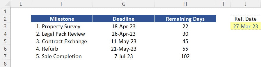
As it stands (i.e. today`s date), your Countdown Calendar is showing that the first milestone is due in less than 1 month (red background colour) which is the urgent one to tackle. The last milestone is the only one due in more than 100 days (green background) while the remaining deadlines are marked with a yellow background which basically alerts you that very soon those milestones will be the critical ones in your project.

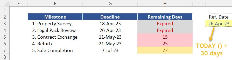
Countdown Calendar at Today`s Date + 30 days:

Now, assume you open this file 30 days from now (i.e. Cell J3 = TODAY() + 30). In that case, no milestone in green will show up anymore, 1 milestone will be on alert, 2 will be the critical ones and the other 2 will expiry by then.

Function NETWORKDAYS

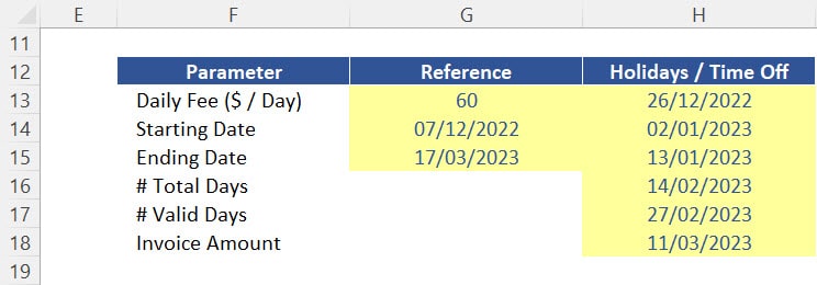
This is straight forward compared to building a countdown calendar. The function NETWORKDAYS calculates the number of days between 2 dates by excluding all weekends and holidays in between. In our example below, let`s assume you are working as a contractor for a company, and you now need to charge that client a daily fee for each day you have worked on a specific project. The invoice amount is basically a daily fee of $ 60 / day times the number of days you have actually worked.

How to work with the function NETWORDAYS:

To fill the table above, follow the steps below:

1. In cell G16, subtract cell G14 (Starting Date) from cell G15 (Ending Date). Here we will get the result 100. Let’s use this as our reference point for the number of days between those 2 dates including all weekends in between.

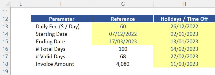
2. Next, we need to calculate the number of days between those dates by excluding the weekends. So, insert the function NETWORKDAYS in cell G17. The first argument “start date” must be cell G14. The second argument “end date” must be cell “G15”. Let’s ignore the argument “holidays” for now. Close brackets and press ENTER. Here we will get the result 73. Therefore, out of 100 days between those 2 dates, only 73 days did not fall on a weekend.

3. Next step is to adapt that function by including holidays or any time off you took during this period (i.e. list of 6 days displayed in column H). So, press “F2” in cell G17 and for the last argument “holidays” select the range H13:H18 and press ENTER. The number of valid days then decreases from 73 to 68.

4. The invoice amount (cell G18) is then basically cell G13 times cell G17.

Function NETWORKDAYS – Bonus Tip:

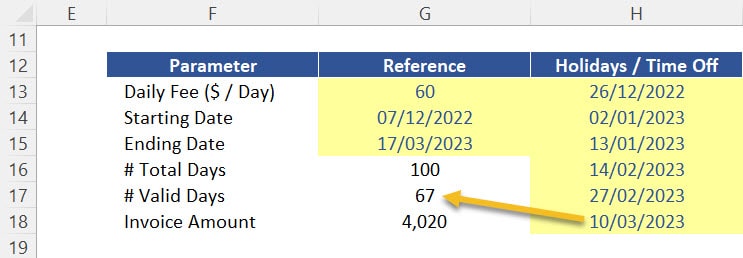
If you paid attention to step 3 above you will notice that the number of Valid Days decreased from 73 to 68 (i.e. decrease of 5), even though the list “Holidays/Time Off” contains 6 days. We did this on purpose to illustrate a key concept behind this function. The function NETWORKDAYS basically excludes from the calculation any holidays or days off which you might have accidentally marked on a weekend.

This is to avoid double counting as the function by default already eliminates weekends based on your computer calendar. To confirm that, change the date 11/03/2023 (a Saturday) to 10/03/2023, which is a Friday. By doing it the number of valid days decreases to 67 and the correct invoice amount should be just over $ 4,000.