Expanding a Drop-Down List:

In part I of this tutorial, we learned how to insert and manage a statical drop-down list. In practice, you are likely to need to add new information to your lists as your dataset at work may evolve over time. Therefore, in this part II you will learn which actions you should take when you need to expand a drop-down list.

Key Issues while expanding your drop-down list:

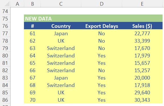
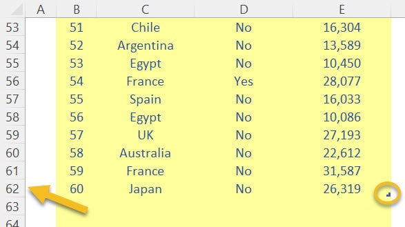
For sake of example, scroll down to the very end of the supporting spreadsheet and you can notice you have now 10 new export entries, including Switzerland which was not part of the original list.

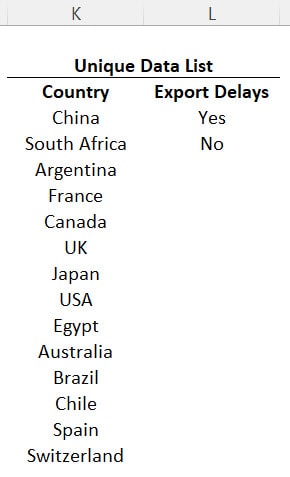
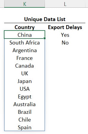
If you go back to the top of your sheet you can see your unique list for countries has still a total of 13 countries and Switzerland is not located anywhere here. Therefore, this country will not show up in your drop-down list either.

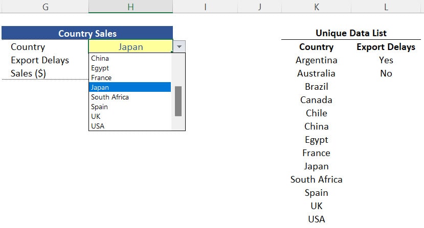
In addition to that if you press F2 in cell H5 you can see that the range arguments of the function SUMIFS end in the row 62 and we know these arguments should change in case we add new information in those additional cells.

With these observations in mind let`s check how we can expand our dataset using a manual and an automatic approach.

Expanding your Drop-Down list – Manual Approach

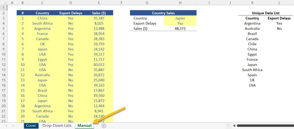
Before we start, let`s create a new sheet by clicking on the plus sign (+) button available at the bottom of your Excel screen and let`s copy all the contents from the first sheet into the new one. Rename the new sheet as “Manual” and remove the gridlines in the Page Layout menu. We can now compare the different approaches we can take when we need to expand our dataset.

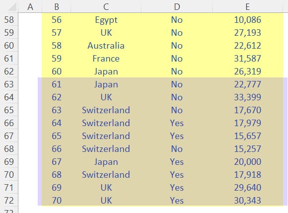
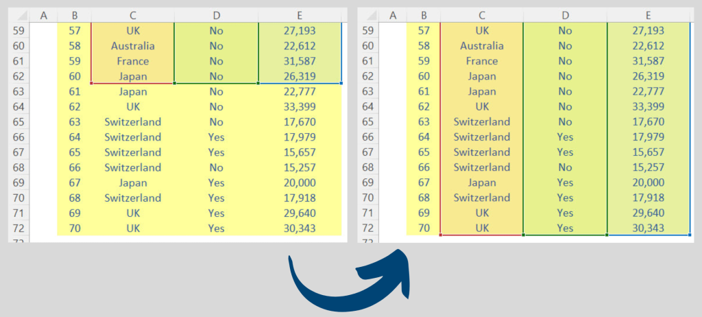
So, to manually expand your dataset, first copy the new data you have at the very end of the sheet you labelled as “Manual” (i.e. “New Data” located in the range B77:E86) and paste (as Values) at the bottom part of your dataset (i.e. cell B63).

After you insert the new data points in our original dataset, the following issues will happen:

Issue # 1 – Function SUMIFS omits adjacent cells:

The function in cell H5 becomes inconsistent and an alert will show up there saying that the function is omitting adjacent cells, which is exactly the case. At the moment, the result of this formula shows total sales for Japan in the amount of $ 48,373. However if you press F2 on it and trace where the range arguments of this function end you will notice they are still ending in the row 62. To correct this issue, manually expand the range arguments of the columns C, D and E.

Issue # 2 – Unique List not updated:

If you go back to the sheet H5 you can notice the results of Japan have increased by $ 20,000. However, if you try to select Switzerland (available in the new data you copied) you will not be able to find in the drop-down list inserted in that cell. This happens because the “Unique List” of countries has not been updated yet. To update it you need again to make some manual adjustments. So, copy the range of column C (i.e. range C3:C72) and paste (as Values) in cell K4. Click again on “Remove Duplicates” (in the menu Data) by keeping the same selection in place. Now, 14 unique cells remain. Your “Unique Data list” for countries is now updated with Switzerland showing up at the very bottom of that list.

Issue # 3 – Unique List not sorted anymore:

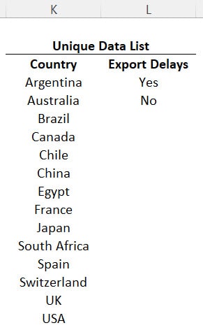
So, as you had to redo the process of creating a new Unique List, you now need to manually sort that data one more time. So, select the range K4:K17, right click, choose “Sort”, and then choose “Sort A to Z” (keeping the current selection in place). Your Unique List will be sorted on alphabetical order from Argentina to USA.

Issue # 4 – Data Validation “Source” not expanded:

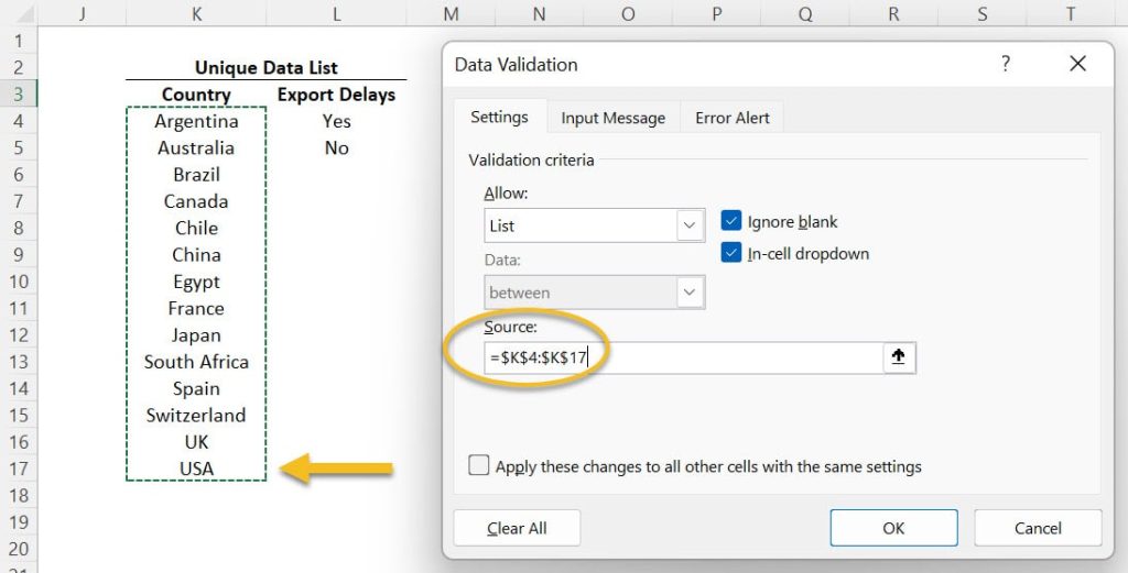
Now if you try to choose the new country “Switzerland” in your drop-down list, you will be able to do so. However, if you try to select the country “USA” you will not be able. This is because your drop-down list was set to end in cell K16 and as you expanded your dataset with 1 additional country, “USA” was pushed one cell down in that range (cell K17) and therefore that cell is not captured by the static drop-down list you built in cell H3. To correct this issue, you need to manually expand the range which is feeding your drop-down list. So, go to the menu Data, click again on the tool “Data Validation”.  In the field “Source”, the new range must be K4:K17 (as you now have 14 unique countries as opposed to 13 before the update).

Your drop-down list is finally updated. However, in case you receive new information you would have to take all these manual steps again which can be too time consuming. Instead, let`s check how to do it automatically.

Expanding your Drop-Down list – Automatic Approach

To make sure your Drop-Down list automatically expands when you receive new data, you just need to follow 3 steps which are all done in advance and only once. So, let`s get back to the first sheet of the file to demonstrate how we can save time and avoid errors.

Step 1 – Getting an Excel Table

The first step is to transform your original dataset into an Excel Table. Follow the steps below:

1. Select any cell of the dataset and press the shortcut CTRL T to create a Table.

2. Make sure the option “My data has headers” is correctly marked in the menu that will pop up and press ENTER.

3. After the Excel Table procedure is inserted, you will gain access to the menu “Table Design”. There you can keep the same format by clicking in the first option in the field “Table Styles” and you can also eliminate the filter buttons for example. You can still recognize your data set is an Excel Table when you look at the right bottom corner of that range. You will be able to see a blue icon on it. And note this is marked in row 62 which is where your dataset currently ends.

This step is complete. By having an Excel Table in place it you can be sure any formulas or functions linked to this range will automatically expand when you add new data. This will be clear when update the sample at the end.

Step 2 – Inserting Array Functions

The second step in expanding a drop-down list is to work with 2 array functions in your dataset. These functions will automatically extract unique lists from your dataset.

Array Function “UNIQUE”

The first one is the function UNIQUE () which is available for Office 365. This function extracts unique values from a range of your spreadsheet. So follow the steps below:

1. Clear the range of column K.

2. In cell K4, insert the function UNIQUE.

3. The only argument you need to worry about in this example is the first one (i.e. “Array”). Therefore, select the range C3:C62, close brackets and press ENTER.

4. Excel will now automatically display an initial list of 13 unique countries.

Now, bear in mind this function is linked to an Excel Table. This means any time you insert new information to your dataset, that function will also update.

Array Function “SORT”:

Note that your unique list is not on alphabetical order anymore. To make sure this sorting is also done automatically while expanding a drop-down list, let`s combine the function UNIQUE with the array Function SORT. Follow the steps below:

1. Just after the equal sign (“=”) in cell K4, type the word “Sort”. Press TAB to select the first function that comes out of the list.

2. The mandatory argument of this function is the argument “Array”. In this case that argument must be the result of the function “Unique” you already have here. Therefore, we can ignore the remaining optional arguments, close brackets and press ENTER.

3. Excel will organize your list of 13 unique countries on an alphabetical order, from Argentina to USA.

Step 3 – Using a hashtag symbol (#) to adapt your data source:

The third step is to adapt the data source feeding your Drop-Down list. So far, your Unique Data List will update after you insert any new data in your dataset. However, the drop-down list still has a static range. To make a test, insert 3 letters “A” in the field “Country Name” at the bottom of the dataset (cell C63). You will note that the country “AAA” is now automatically showing up at the very top of the Unique Data List. This means “USA” again was out of the initial range K4:K16, which you defined as the initial data source. You can double check that by expanding the drop-down list of cell H3 and confirming “UK” is the last country name. To correct that, follow the steps below:

1. Select cell H3 which contains the Drop-Down list.

2. In the Data menu, choose again “Data Validation” and let`s work on the field “Source”.

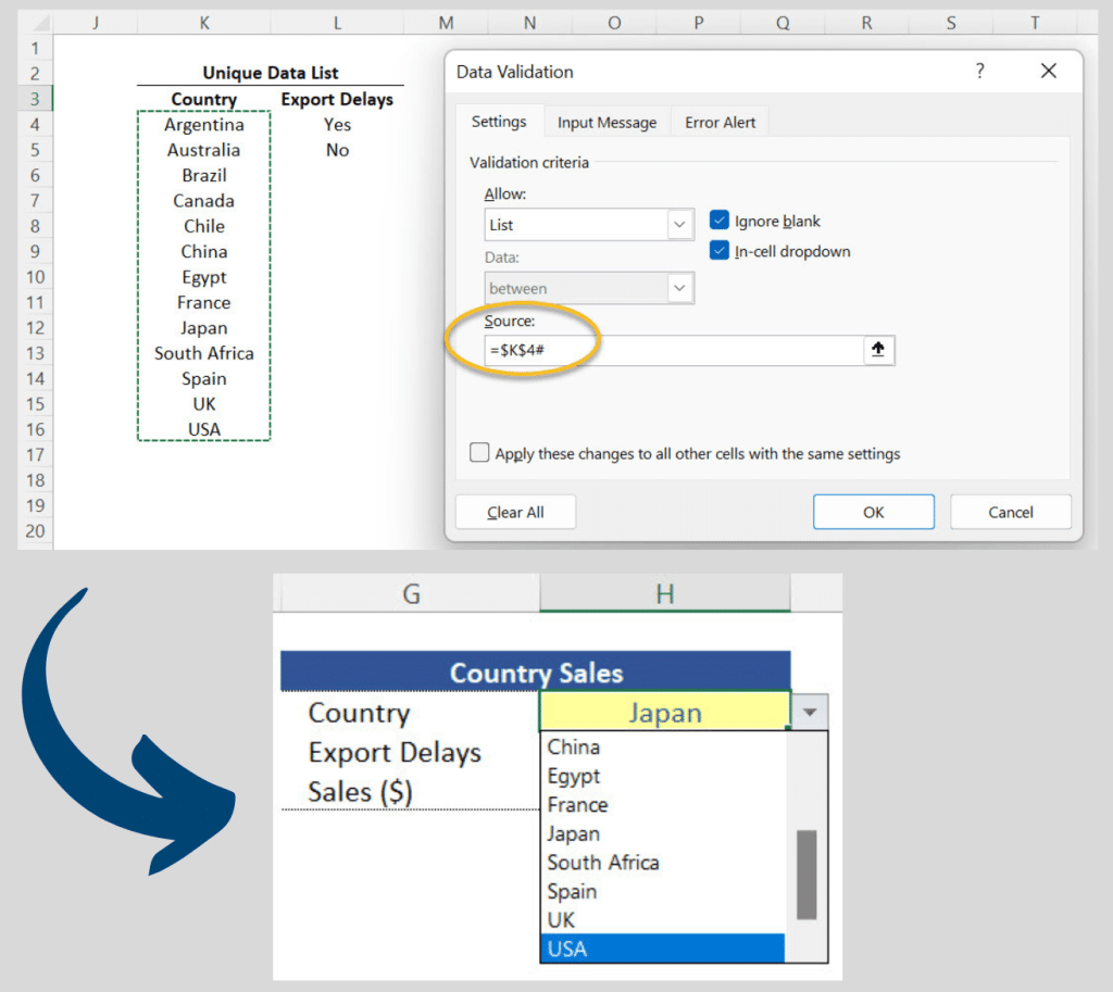
3. To make the “source” automatically expand, whenever your unique list expands, select the first cell of your unique list and insert a hashtag symbol (#). This is the way Excel can understand you are linking your source to an Array Function which is the case here.

4. You can confirm that the drop-down list is now showing you “USA” as the “Source” of your Drop-Down list has also automatically expanded this time.

Testing your new drop-down list:

We have just completed all 3 steps to create an automatic drop-down list. So, let`s complete our initial example by copying again the range B77:E86 and pasting it (as Values) in cell B63. We can observe the following:

a) Sales form Japan, as expected, have automatically increased by $ 20 k. This happened without any manual adjustment in the function SUMIFS.

b) Switzerland didn`t show up in the Unique List when we took the manual approach. However, now you can see that country in cell K15.

c) The Unique List automatically sorts itself on alphabetical order.

d) After expanding the drop-down list of cell H3, we can see USA at the bottom of the list.

So, in summary, you organize your data in advance by preparing your Excel file through these 3 steps. You will then be able to add new information to your data source and the outputs will update automatically. More time saved to you!