Function IFERROR:

Let`s now check 2 practical examples on how and when to use the function IFERROR.

Example 1: “Text” instead of “numbers” in your dataset

In this first example, we need to identify the total variable cost incurred by each of these companies from A to P. For each business, we have the Volume Sold of a specific product as well as the Production and Delivery costs. Total Variable Costs for company A for example should be equal to the Volume Sold from cell C5 times the sum of Production (cell D5) and Delivery costs (Cell E5). After inserting the first formula, you can then expand it down to entire range, you will note 4 error alerts will come out in the screen.

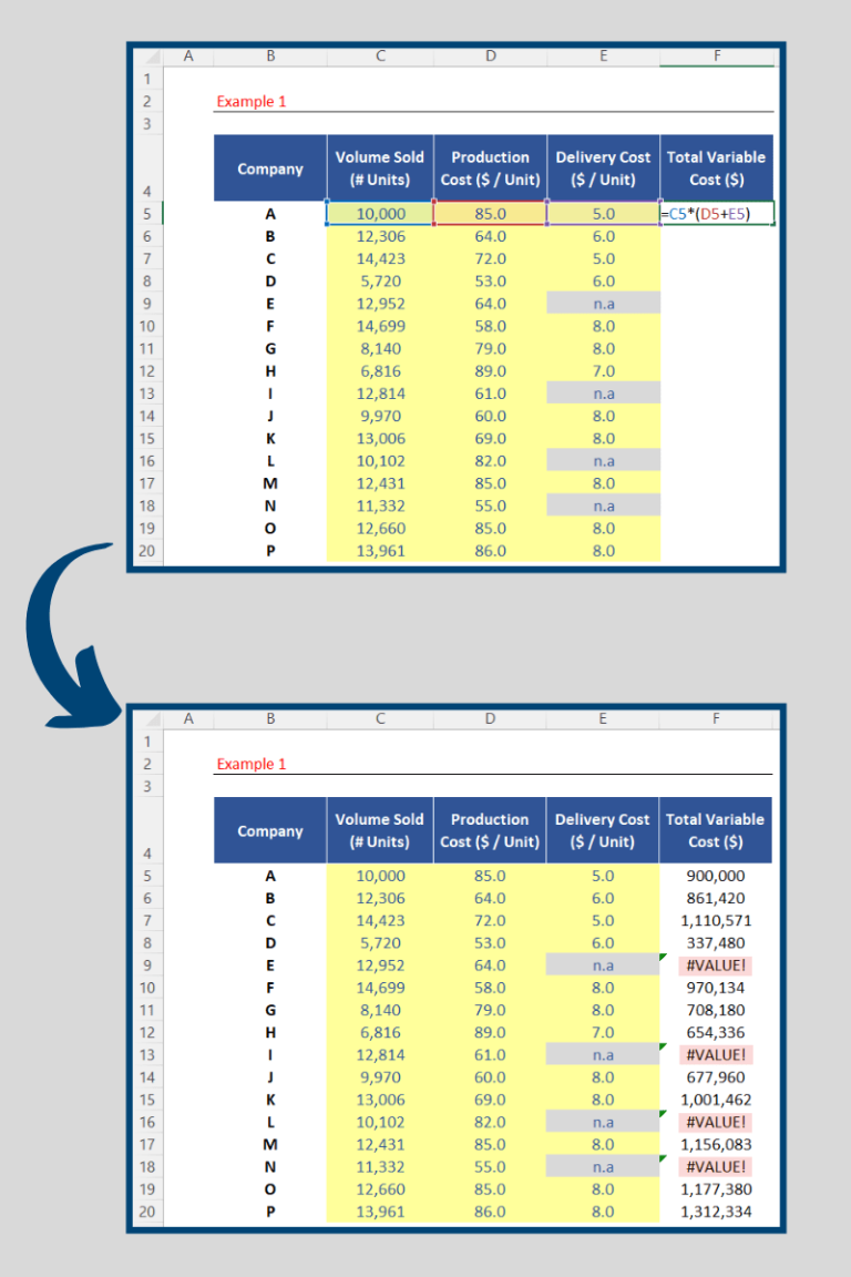
The error type above is known as “Error in Value” because one of the parameters used in this multiplication we created is actually not a value. This was the case for companies E, I, L and N. As there`s no information related to “Delivery Costs” for these companies, the “non-applicable” notation was inserted in those cells which creates the multiplication error.

Example 1 – Correcting the formula with the function IFERROR

To correct this issue, we need to have an adapted formula for each of these companies which have this error alert displayed. The adapted formula should then be limited to the variables Volume Sold times Production Cost only. However, you don`t want to waste time adapting your calculations anytime you identify an error in the original formula. That`s the moment where you need to work with the function IFERROR. Follow the steps below:

1. Press F2 in this cell F5 and just after the equals sign type the word IF.

2. The function IFERROR is in the second position of this list, so highlight that option and press TAB to select it.

3. This function requires 2 arguments. “Value” and “Value If Error”. The argument “Value” is basically the result of the main formula you are trying to insert. Now press “comma” to skip to the next argument (“Value if Error”). Here you need to disclose what alternative formula you should have anytime the main formula returns you an error.

4. The alternative formula in this case should be “Volume Sold” multiplied by the variable “Production Cost” only (i.e. C5 multiplied by the cell D5 only).

5. Expand the formula down to all cells of the range.

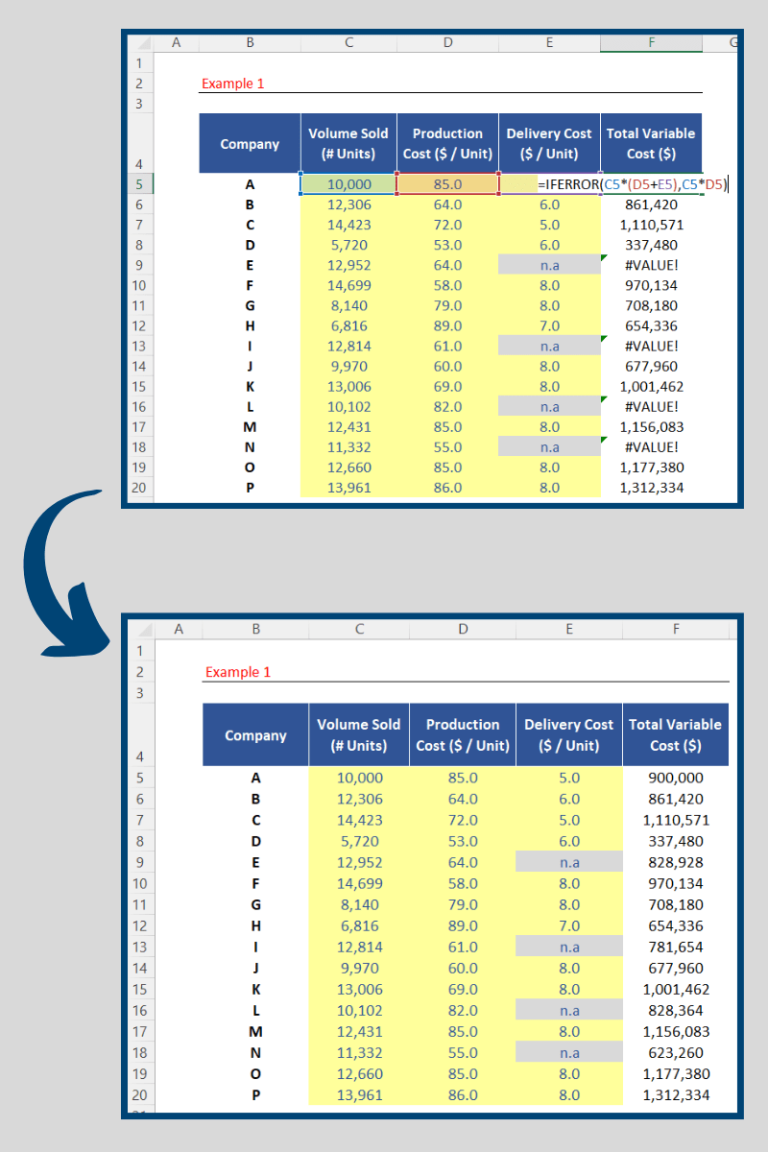
By doing this, you are creating an automatic adaptation in all of your formulas. In other words, if you have a valid data point for the variable Delivery Cost, then that data point will be part of your calculation. If that`s not the case, we then need to exclude that variable.

Example 2: Errors coming from a division formula

In this second example, we need to calculate the Profit Margin for each business. This is a metric which basically shows what portion of the revenues has been successfully transformed into a profit which is done with a simple division. We can then perform that calculation for company A in the cell K5 and again send it down to the remaining cells of the range, and 3 error alerts will appear.

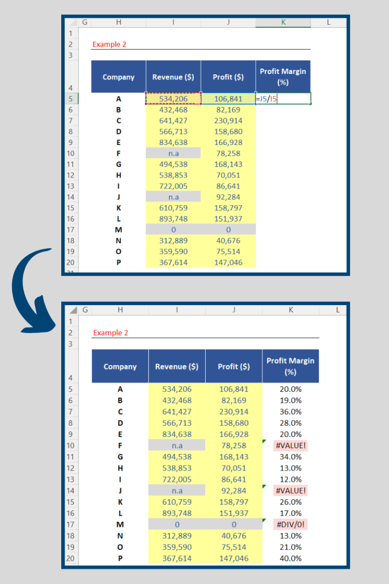
The first 2 errors are classified as “Error in Value”. This is because again we have the notation “non-applicable” in those cells. As this is a text and not a value itself, that error alert will pop up. The third error is the “Divide by Zero” error. It shows up because it`s impossible to divide any number by zero.

Example 2 – Correcting the formula with the function IFERROR

Regardless of the type of error we find we need an alternative result to show up here so let`s again use the function IFERROR (). Follow the steps below:

1. Press F2 in this cell K5 and just after the equals sign type the word IF.

2. The function IFERROR is in the second position of this list, so highlight that option and press TAB to select it.

3. The first argument “Value” is the original formula itself, so press comma to skip to next argument. This is then the value you will get in case you find an error in your division. Let`s assume you want “zero” for this argument, so we can complete this function.

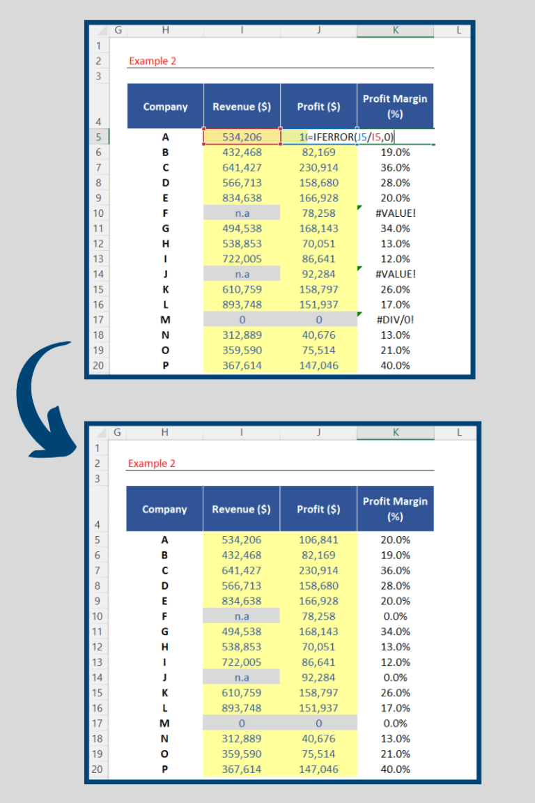
By taking this approach you will automatically replace any errors arising from your formula by a number zero.