Function LEN

The function LEN (or “Length”) serves to return the total number of characters in a text string and it will consider the spaces and punctuation, but it will ignore the format of the text. Another key point is that the only argument required is the text you are working with.

Function LEN – Basics

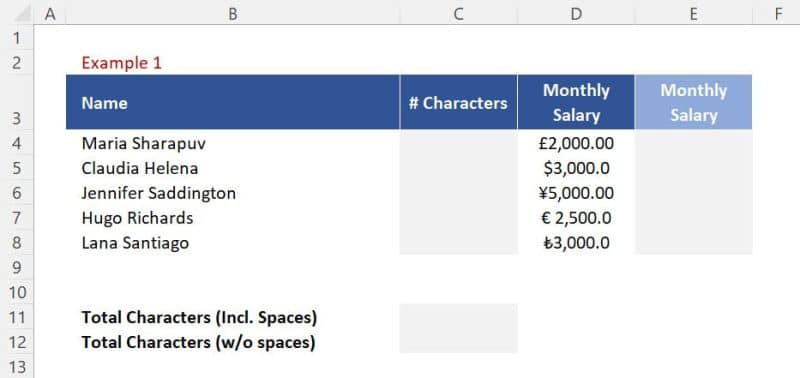
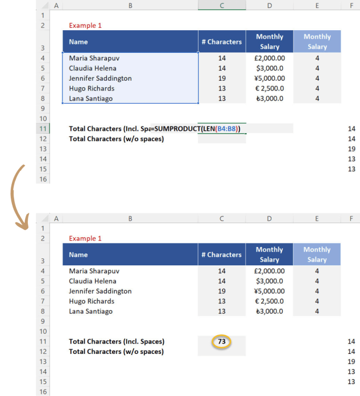
In example 1 below, we have a list of names, and we want to know how many characters there are in each name.

To do that, let’s work with the LEN function:

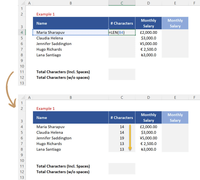
1. First, go to cell C4 and insert the function LEN.

2. After that, select the “text”, which in this case is cell B4.

3. Finally, close brackets and press ENTER. The result will be 14, which represents the number of characters in the name “Maria Sharapuv”, including the space.

If you expand the function, you will have the number of characters for the rest of the names as well.

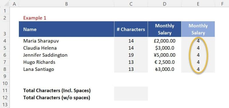
But what happens when you’re working with formatted text? Well, it basically ignores it and we can demonstrate that. In example 1, we also have a monthly salary for each of the names and the text, in this case, is formatted. If you repeat the process explained above to get the number of characters of the salary “£2,000.00”, the result will be 4 even though we have a pound symbol (£), a thousand separator, and decimals here. Expand the formula to the rest of the rows; the result will also be 4, because the LEN function doesn’t take text format into account when calculating the number of characters.

Function LEN – Number of characters with and without spaces

Continuing with example 1, let’s learn how to get the number of characters with and without spaces:

1. First, go to cell F11 and insert the LEN function.

2. Next, select the entire array of names from B4 to B8.

3. You can then close brackets, press ENTER, and the result is an array with the number of characters from the list of names of the table above.

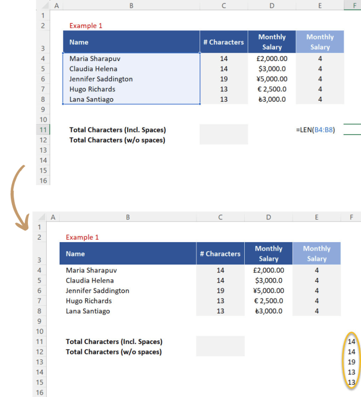
This procedure is very useful as it allows us to make calculations for an entire array if you can’t add a helper column right next to our data set.

Number of Characters with Spaces:

Now, let’s get the number of characters with spaces:

1. First, copy the LEN function you just made after the equal sign.

2. Go to cell C11 and insert the function SUMPRODUCT.

3. Next, paste the LEN function to use it as the argument “array 1”.

4. Finally, close brackets and press ENTER. The result is 73, which is the total number of characters for all 5 names, including spaces.

And this is basically how you can work with arrays when using the LEN function.

Number of Characters Without Spaces:

However, you might also need to get the number of characters without spaces. For that, you must work with the SUBSTITUTE function:

1. First, go to cell F11 and insert the SUBSTITUTE function.

2. Next, for the “text” argument, select the entire range of names from B4 to B8.

3. After that, press comma and then, for the “old text” argument, open quotation marks, add a space, and close quotation marks.

4. Press comma again and add two quotation marks (this time without any space in between) as the “new text” argument.

5. Finally, close brackets and press ENTER.

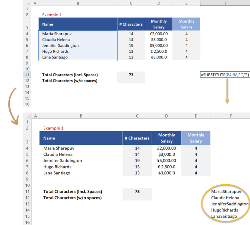
What we just did is replace the “space” with “no space”. By doing it, we could basically obtain a list of names without any spaces.

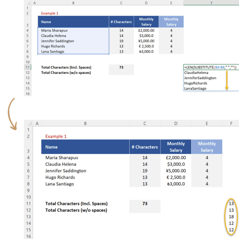
Next, you can edit the SUBSTITUTE function by embedding the function LEN (after the equal sign) and adding another bracket at the end of the formula. Press ENTER and now you have the number of characters without spaces for the entire array.

Now follow the steps below to finish the process:

1. So, copy the entire function after the equal sign.

2. Go to cell C12 and insert the SUMPRODUCT function.

3. Paste the function LEN to use it as the “array 1” argument.

4. At last, close brackets, press ENTER, and the result is 68, which represents the total number of characters for all the names in our list without including the spaces.

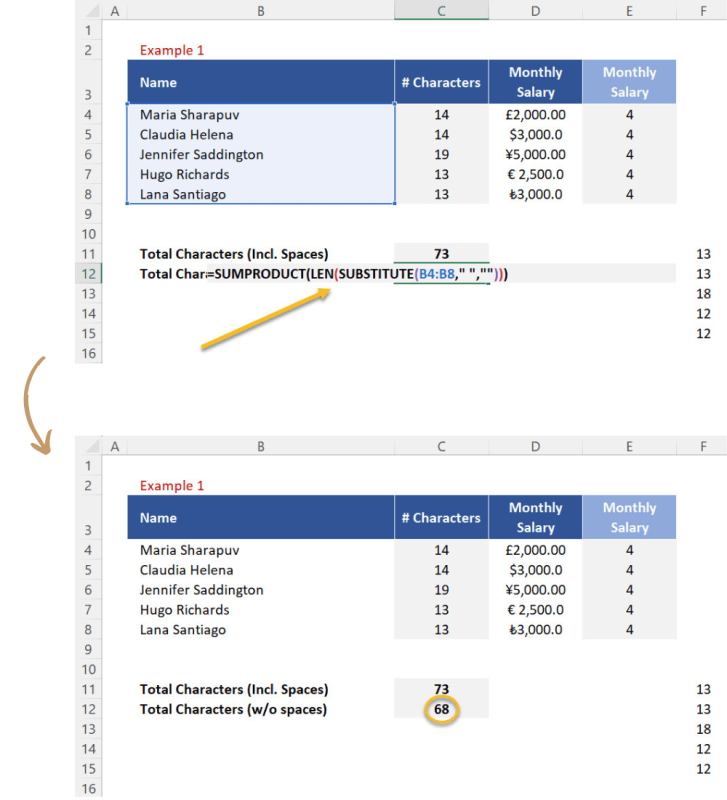
This can be quite useful when you need to work with sentences in Excel for tasks which impose restrictions around the maximum number of characters you can use.

Function LEN: Support to Flash Fill

The command Flash Fill allows us to extract a specific piece of data from a sentence. However, in specific situations like in this example 2, it might not work. In example 2, Here we have a dataset, and we need to extract the purchase year from each input. In each data point, the first number represents the month, and the next 4 numbers represent the year. Of course, some months have 2 digits, like 11 for November and 12 for December, and that makes it less logical for Excel to understand the pattern.

Normally, Excel users would manually extract the purchase year of each data point:

1. So, go to cell H4 and type 2023.

2. Then, go to cell H5 and type 2024.

3. Now, expand the formula by selecting cells H4 and H5 and dragging them down to cell H9 to get the results for the entire range.

4. Finally, go to the AutoFill menu and click “Flash Fill”.

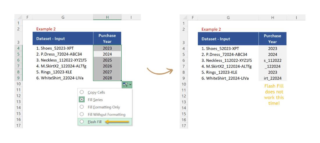
As you can see, Excel will automatically extract the data. However, we get a lot of errors because our dataset is not standardized, and therefore Flash Fill will not work well in this case. Let’s delete these calculations and move on to fishing the issue.

Flash Fill workaround:

In situations like this, we must find a common element in our dataset to use as a reference. But first:

1. Go to cell I4 and insert the function LEN.

2. Then, open brackets, select cell G4, close brackets, and press ENTER. The result in this cell is 18, which is the number of characters in the first data input in our table.

4. Finally, you can then expand the function down to cell G9 to get the number of characters for the rest of the inputs.

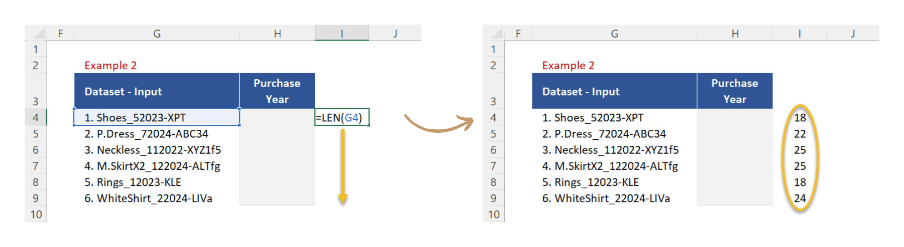
We will use this formula later. But first let`s complete an important step!

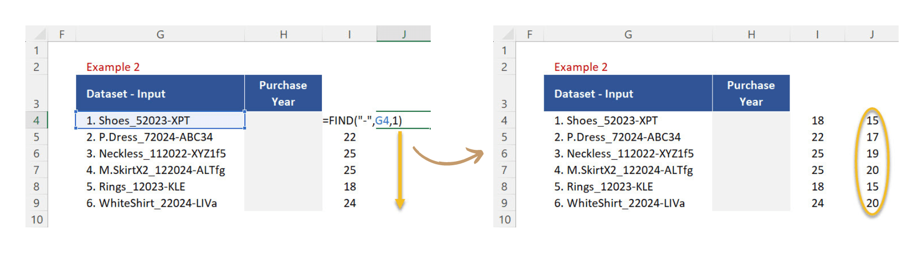
Workaround – Finding a “Common Element”

If you look at the table we have, you can see that a “common element” in our database is the hyphen, which is located after each variable “year”. Let’s use the FIND function:

1. So, go to cell J4 and insert the FIND function.

2. For the argument “find text” you need to open quotation marks, press hyphen, and close quotation marks.

3. Now, for the argument “within text”, select G4, and press comma.

4. After that, add 1 as the “start number” argument, which refers to the position from left to right where the assessment will be done.

5. You can then close brackets, press ENTER, and the result is 15, which represents the position of the hyphen within the first data input.

6. Finally, expand the function down to cell J9 just so you get the results for the rest of the rows.

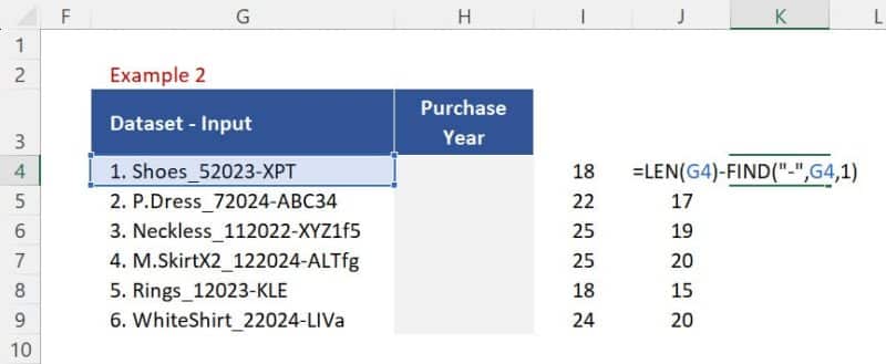
The next thing to do is to get the difference between the results of these functions. Follow the steps below:

1. In cell K4, insert equals (“=”) and make the difference of cell I4 (i.e. total number of characters) minus cell J4 (i.e. position of the hyphen from left to right in the given code of cell G4).

2. Next, copy the function LEN after the equal sign and use it to replace the argument I4 of the formula you just inserted above.

3. Finally, copy the function FIND and use it to replace J4 after the minus sign of the same formula.

Workaround – Using the Function RIGHT

Copy the entire nested function from the previous step (after the equal sign) and follow the steps below:

1. Go to cell H4 and insert the RIGHT function, which tells Excel to extract a certain number of characters to the right of a sentence.

2. For the argument “text”, select cell G4 and press comma.

3. Next, paste the nested function we just copied because we need to use it as the “number of characters” argument.

4. Close brackets, press ENTER, and the result is “XPT”, which are the three characters after the hyphen.

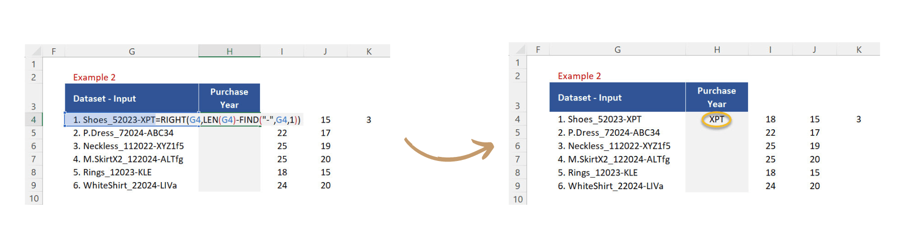
If we go back to the formula and we add 1 at the end, the result will now also include the hyphen, because we are asking the function to extract 1 more character on the right of the text. Using the same logic, if we now add 5 instead of 1, we will also get the “year” which is composed of 4 digits.

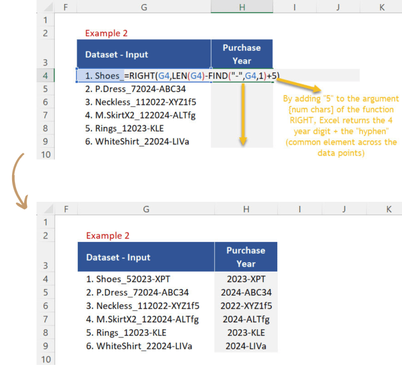
Expand this to the rest of the rows and delete the helper columns.

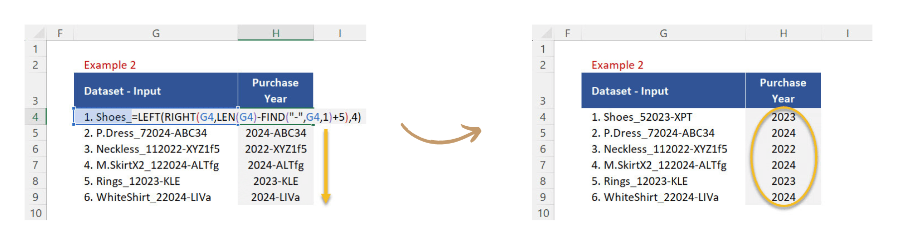
Workaround – Using the Function LEFT

Now, we can do a similar thing with the function LEFT, which extracts a certain number of characters to the left of a sentence in this case:

1. Go back to the function and insert the LEFT function.

2. The “text” argument will be the formula that’s already there while the second argument must be 4, as we need the 4 digits which makes a year.

4. Finally, press ENTER and expand the function to the rest of the rows.