Function TEXTJOIN

This is a straight forward Excel function. Let`s check a basic example and a few variations of the function TEXTJOIN.

Function TEXTJOIN – Basic Example

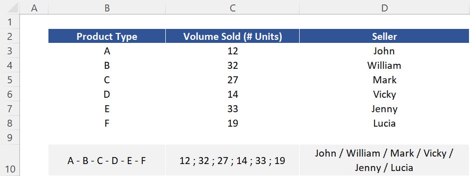
In this example, we have 3 pieces of information related to the sales of items made in a store: (a) Product Type, (b) Volume Sold and (c) Seller. Our task is to gather the information contained in each of these 3 columns and display the combined results in the respective cells of row 10.

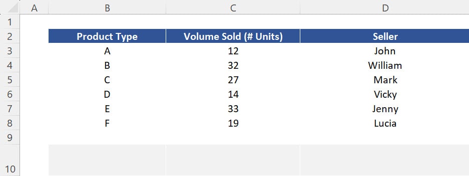
This can be done with the function TEXTJOIN. Follow the initial steps below:

Working with the function TEXTJOIN:

1. So, insert the function TEXTJOIN in cell B10.

2. After that, the first argument is the “delimiter”. Here you can basically use whatever you want. However Excel users normally select delimiters such as comma (,), semicolon (;), dash (-), underscore (_) or forward slash (/) for instance. For now, let`s leave this argument as “empty” meaning that any data we select going forward will be concatenated only. Press comma to skip to the next argument.

3. The argument “Ignore Empty” is used if you want the function TEXTJOIN to ignore empty arguments from the column containing the information you need. At this stage, let`s select the option “TRUE” for this argument and press comma.

4. Next we have a series of “text” arguments. This is basically the cells from column B which we need to get together. Here you can select these arguments one by one or select the entire range B3:B8 at once to save time. You can then close brackets and press CTRL + ENTER.

5. Finally, expand the same function to the entire range B10:D10.

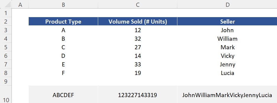
Inserting a “delimiter”:

All the data has been concatenated. However, this is not yet looking nice. Even though the data of each column is now located in one cell only, it`s really hard to identify the strings individually. That`s the reason you need a delimiter. So, follow the steps below:

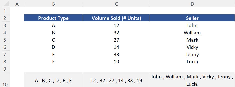
1. So, press F2 in cell B10. For the first argument “delimiter”, let`s insert a comma (,) with spaces, but make sure to use quotation marks (“ “) otherwise your function will not return you a correct result.

2. You can then press CTRL + ENTER and expand the same formula to the entire row. We can now clearly identify all the strings.

Function TEXTJOIN – Bonus Tips:

Now, 2 tips to handle this function.

Bonus Tip 1: Argument “Ignore Empty”

First, let`s check the impact of changing the argument “Ignore Empty” in the function TEXTJOIN. Follow the steps below:

1. First, press F2 in cell B10 and change the argument “Ignore Empty” from “TRUE” to “FALSE”. By doing this function will not ignore empty strings anymore. Copy that function to the entire row 10.

2. You can then press ENTER and then select the region B5:D7, cut it (CTRL + X) and paste it (CTRL + V) in another area of your spreadsheet. As expected, empty strings will show up in the results displayed in row 10.

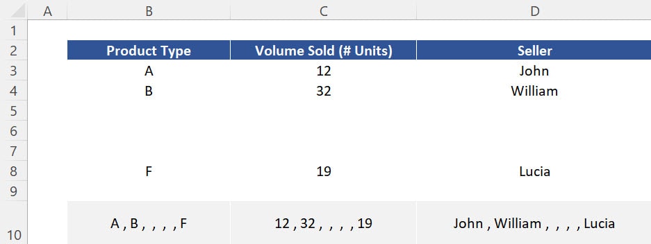
Unless you need to demonstrate empty strings for a specific task at work, keep the argument “Ignore Empty” as “TRUE”. With this in mind, press the shortcut CTRL + Z three times to undo the previous 3 actions.

Bonus Tip 2: Correct “delimiters”

The second tip is around the delimiters to be used. Try to test different delimiters and choose the one that looks better for each data type you have. We need to correct that with the following steps:

1. So, in the function of cell B10, let`s change the argument “delimiter” from a “comma” (,) to a “dash” (-).

2. After that, in the function of cell C10, let`s change the argument “delimiter” from a “comma” (,) to a “semicolon” (;).

3. Finally, in the function of cell D10, let`s change the argument “delimiter” from a “comma” (,) to a “forward slash” (/).

Your results should look like the image below.