Paste Special – Advanced Tips

Now that you understood the basics of Paste Special (covered in the part I of this tutorial), let`s check some Advanced Paste Special techniques you need to know to apply at your work.

Data Transposing (Turning rows into columns and vice versa)

The tool Paste Special can also be a huge time saver when you need to transpose an information in your spreadsheet. For example, the table below displays the products vertically where each product price is located in a different column.

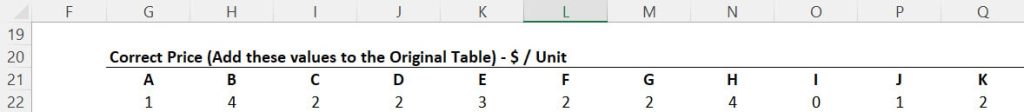
To transpose that information you can then copy the range G21:Q22 and then:

1. Select an empty range of your sheet such as the one starting in cell G3.

2. Press CTRL ALT V to open the “Paste Special” menu.

3. Select the option “Transpose” and press ENTER. Excel then automatically transposes that information to you.

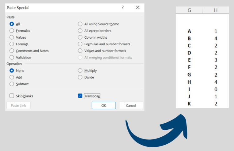
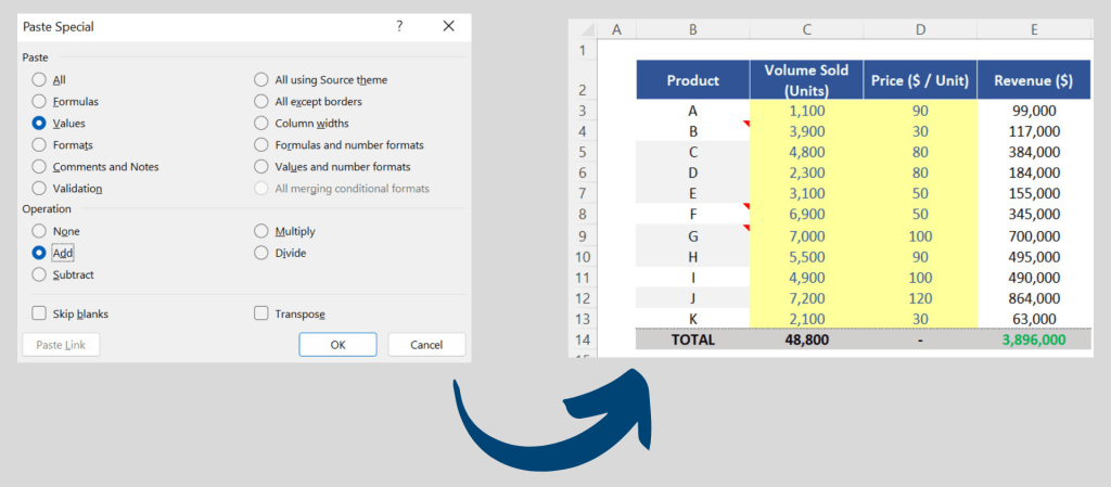
So, all information originally displayed in the rows will now be displayed in the columns, and the same from the columns in the rows. Once you have your information correctly located side by side you can then easily work with your dataset. For example, here let`s assume we need to add this series of prices to the original prices displayed in column D of our reference table. Follow the steps below:

1. Select the range H3:H13 and copy it.

2. Select the cell D3 as a reference point, press CTRL ALT V to open the Paste Special menu.

3. Select “values”, and then select “Add” for the math operation and press ENTER. All prices of this column D will increase by the respective values you displayed in the column H.

Skip Blanks (Advanced Paste Special tip for ordinary tasks in Excel)

Now, copy the information related to Volume (range G17:Q18), select cell G3 again, press CTRL ALT V and click again on “Transpose”. That information will be transposed to you.

Note that as we decided to copy all elements of the original range, the grey background colors (representing blank cells) were also copied which is fine for this example. We now need to correct the Volume information related to the products C,D,E,G, H and J in our original table (column C). Bear in mind that any other products should keep their initial values in place.

And here`s the tricky part. If you just try to copy the values from column H and paste in column C (by using CTRL +C / CTRL + V), all blank cells will be copied and pasted which is wrong!

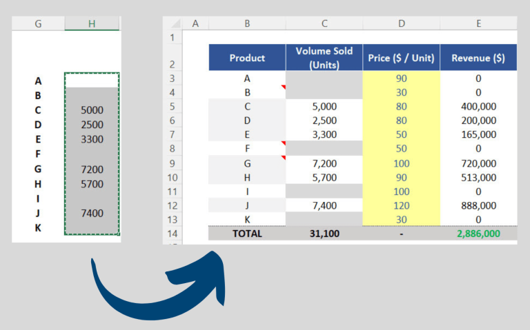
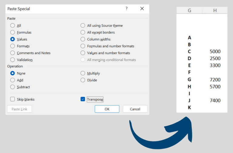
So, press CTRL Z to undo this action. The correct approach in a situation like this is to make sure you copy the entire range but excluding the blank cells. To do that, follow the steps below:

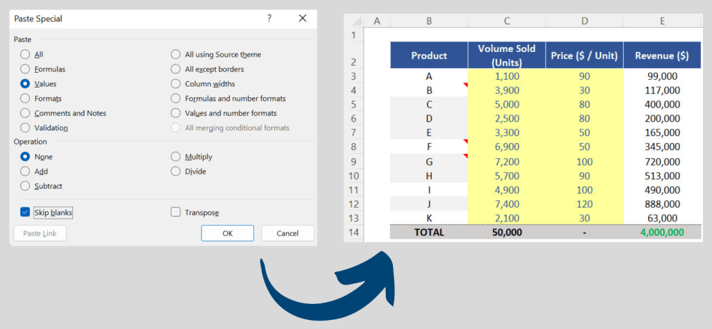
1. Select again the range H3:H13 and copy it.

2. Select the cell C3 as a reference point but now press CTRL ALT V to access the Paste Special menu.

3. In that menu, select the option “Values” as you need to keep the original format in place, but this time make sure you click on the option “Skip Blanks”. By doing this, you are basically ignoring any blank cells you copied before. If you press ENTER, only the cells which indeed had a value will replace the respective original data from column C.

Paste Link (Advanced Paste Special for quick links in your workbook)

If you now click on the second sheet of the downloadable Excel file (“Paste Special_Chart”), you can see we have a table which we need to complete. We also have a chart which is linked to the data related to the Volume your company was expecting to sell during the year. The first thing we need to do here is to make sure all the information that needs to be displayed in this column C is linked to the first sheet of the file (“Paste Special_Basics”). The easiest way to perform this action is by doing the following:

1. Go back to the first sheet (“Paste Special_Basics”).

2. Select the range you need which in this case is the range C3 to C13.

3. Press CTRL C to copy it and go back to the second sheet (“Paste Special_Chart”).

4. Select cell C3 as a reference point.

5. Now, press CTRL ALT V and on the button called “Paste Link”. This entire range will be linked to the original sheet, so any changes you make in the first sheet will be automatically reflected on the second one, which helps you to avoid duplicated work in your Excel files.

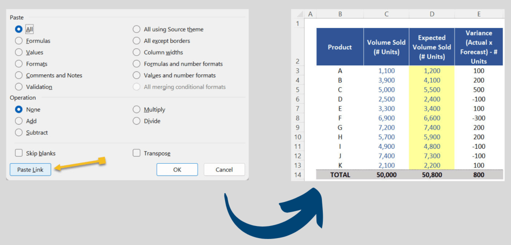
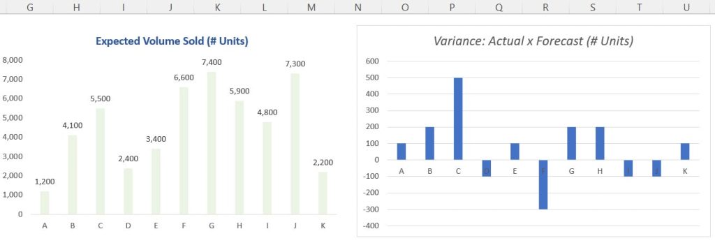
Now you can see the Actual Volume Sold against the Expected Volume Sold. To calculate the variance between them, insert a simple formula in cell E3 where you subtract for each value from column D the respective value from column C and then send down the function.

So, in total, your company was expecting to sell 50,800 units of a specific product and it actually sold only 50,000 units. We can explain this difference of 800 units when we look at the variance calculation we performed to each product above.

Updating a Chart Format (Secret Weapon)

This is another import Advanced Paste Special command you must know. The last task we need to perform here is to create a similar chart to this one below which must show the variance calculation from column E.

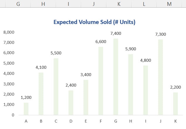
Follow the steps below to quickly insert the new chart you need:

1. Select columns B and E simultaneously (i.e. by holding the CTRL key).

2. Press the shortcut ALT F1 to insert a new chart and position both charts side by side.

3. Change the title of the second chart to “Variance: Actual x Forecast (# Units)”. The idea here is to replicate the same chart style from the first chart into the second one.

At a first glance, we can spot many differences between the charts. For example, the first chart does not have any gridlines, or any borders and the information is clearly displayed with data labels among many other differences. For a task like this, you can also use the tool “Paste Special”. Follow the steps below:

1. Click on the first chart.

2. Press CTRL C to copy all the elements of that chart.

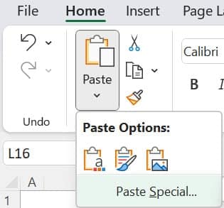
3. Select then the second chart and this time go back to the “Paste Special” menu on the top left corner of your screen (explained in the part I of this tutorial).

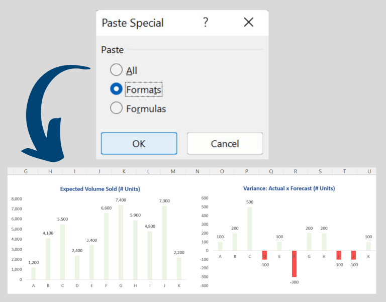
4. There, you just need to mark the option “Formats” and press ENTER. By doing this, you will get the exact same formatting, including the default option for negative values in the series.