Unique List:

Let`s check through 3 practical examples how you can use the tool “Remove Duplicates” to create a Unique List in your Excel file.

Unique List Definition:

In this example we need to review the sales performance of a group of sales people of a store. In our dataset we are able to see 4 variables: (a) Day of the month when the sale took place, (b) Name of the Sales Executive who did the sale, (c) Product Sold (TV, Mobile, Laptop, etc.) and (d) the final price achieved for each sale ($/Unit).

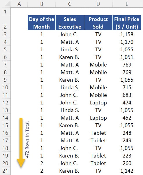
To understand the sales performance of this store, we need to identify the “segments” of our dataset. For example, we can see the name “John” and the product “TV” repeated many times in the extract above. It would be better if we could have a breakdown of sales for every sales person and every product available. We therefore need to identify a “Unique List” of sales people and a “Unique List” of products available, which can be done through the tool “Remove Duplicates”. Let`s check 3 different examples to understand how to do it.

Example 1 – Creating a Single Unique List:

Let`s start by copying the contents of column C and pasting in cell G3 for now. Now follow the steps below:

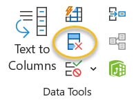
1. First, select the contents of column G and then go to Data and click on the icon “Remove Duplicates”.

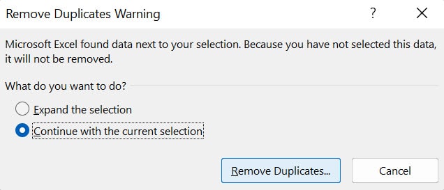
2. At this point, you only selected column G, so the message box below will pop up asking if you want to expand your selection to incorporate the variable “Number of Items Sold” (column H). As this is not the case for this example, simply mark the option “Continue with current selection” and click on “Remove Duplicates”.

3. Next, click on “OK” in the following menu.

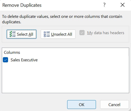
4. Finally, Excel will then display a message saying that “466 duplicate values were found and removed and only 4 unique values remain“.

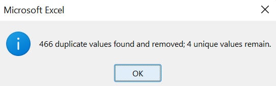
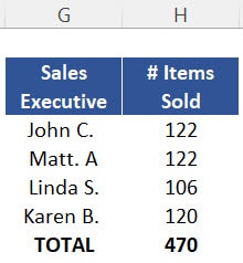
Therefore, a total of 4 unique sales people work in this store (i.e. John C., Matt. A, Linda S., and Karen B.).

Example 1 –  Unique Values & Function COUNTIF

With a unique list of values like this you can perform calculations much easier. In this case, let`s calculate the total sales achieved by each sales executive during this period which can be done with the function COUNTIF. Follow the steps below:

1. Insert the function COUNTIF in cell H3.

2. For the argument “Range”, select the range C3:C472.

3. Now, for the argument “Criteria”, select cell G3 which represents sales person John C. in this case.

4. Close brackets and press ENTER. The result will show that sales agent John C. sold 122 products during that period.

5. Press F2 in cell H3, select the argument “Range” and press F4 to apply “absolute reference” for the column and rows of that range.

6. Copy and paste the same function until cell H6.

7. Type “TOTAL” in cell G7 and in cell H7 press the shortcut “ALT =” to insert the command “Auto Sum” in that cell. Total sales of 470 products were done in the store.

8. Finish the table by selecting the range G7:H7 and pressing the shortcut CTRL B to insert the “Bold” style in that range.

Example 2 – Another Single List:

Let`s repeat the same logic for the variable “Product Sold”. Follow the steps below:

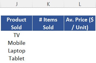
1. Firstly, copy the range D3:D472 and paste it in cell J3.

2. Next, press CTRL A to select the entire new dataset (i.e. columns J, K and L).

3. Again go to the menu Data and click on the option “Remove Duplicates”.

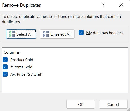
4. As you have noted, this time Excel has not asked if you want to expand your dataset. You already did it in step 2 above. So, in the menu that pops up, select the variables you want to use to generate a unique list. In this case, as we only need “Product Sold”, unmark the options “# Items Sold” and “Av. Price ($ / Unit)”.

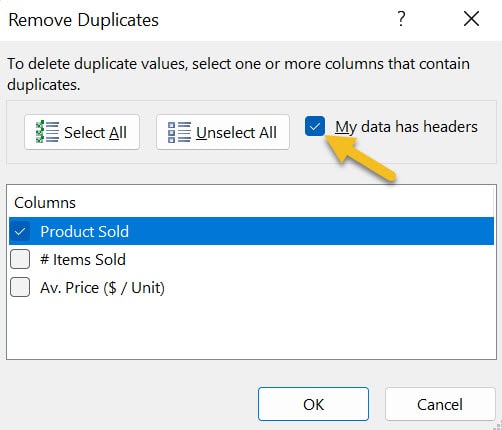
5. At this point, make sure the field which says “My data has headers” is marked as this is the case in this example. If you have a header and you forget to mark it, Excel will basically consider the title of the column (i.e. first data point of your selection) as a unique data point to be filtered as well, which is wrong.

6. Finally, you can then click on “OK” and a message will pop up in the screen saying “466 duplicate values were found and removed, and 4 unique values remain”. You can then press ENTER and check the list of unique products sold in the store (TV, Mobile, Laptop and Tablet).

Example 2 –  Unique Values & Function COUNTIF

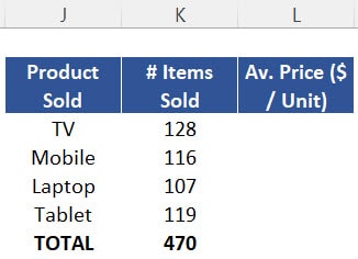
Let`s now count how many products of each category were sold and the respective average price. For the variable “# Items Sold”, follow the steps below:

1. So, insert the function COUNTIF in cell K3.

2. You can then select the range D3:D472 for the argument “Range”.

3. For the argument “Criteria”, select cell J3. Close brackets and press ENTER. Here you can confirm the store sold 128 units.

4. Now press F2 in cell K3, select the argument “Range” and press F4 once to apply absolute reference to it.

5. Copy that formula to the entire range K3:K6 so you can check the total products sold for all categories.

6. Now type “Total” in cell J7. Insert the “Auto Sum” command in cell K7 (shortcut ALT + =). A total of 470 units were sold which matches the result of the first example.

7. Finally, highlight the range J7:L7 with a bold style by selecting that range and pressing CTRL B.

Example 2 –  Unique Values & Function AVERAGEIF

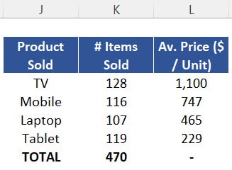
To calculate the “Average Price”, follow the steps below:

1. So, insert the function AVERAGEIF in cell L3.

2. After that, for the argument “Range”, select again the range D3:D472.

3. You can then select cell J3 for the argument “Criteria”.

4. For the argument “Average_Range” select E3:E472 and press ENTER. You can then see TV sets were sold at an average price of $ 1,100 in this store.

5. Now press F2 in cell L3, select the arguments “Range” and “Average Range” and press F4 to apply Absolute Reference on them.

6. At last, expand the function you created to the entire range L3:L6. There`s no need to insert a sum at the of this range so just type “-“ in cell l7.

Example 3 – Creating a Combined List

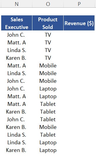
So far we created a unique list for the names of the Sales Executives and a unique list for the Products Sold. However, what if you want to know how much revenue each of those sales executives generated for each type of product? Well, if that`s the case, you basically need to identify a unique combination of these 2 variables and the rest of the process is very similar to what we have done so far. Follow the steps below:

1. At first, select the range C3:D472 (i.e. columns “Sales Executive” and “Product Sold” together). Copy and paste it in cell N3.

2. You can then select the range N3:O472 and go to the menu “Data”. Click again on “Remove Duplicates” and click on OK in the message box which will pop up.

3. At this instant, you will see another message saying “454 duplicate values found and removed; 16 unique values remain”. These 16 unique values are actually 16 unique combinations of “Sales Executive” x “Product Sold”.

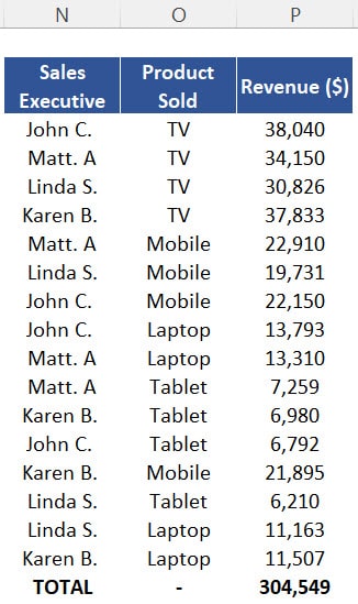
Example 3 –  Unique Values & Function SUMIFS

You have just mapped all the possibilities here, so let`s then calculate the total revenue of each one of them. Follow the steps below:

1. So, insert the function SUMIFS in cell P3.

2. You can then select the range E3:E472 for the argument “Sum Range”.

3. After that, for the argument “Criteria Range 1”, select the range C3:C472.

4. Next, for the argument “Criteria 1”, select cell N3.

5. Now, select the range D3:D472 for the argument “Criteria Range 2”.

6. You can then select cell O3 for the argument “Criteria 2”.

7. After that, press ENTER and you will confirm sales agent John C. has sold $ 38,040 worth of TV Sets in that period.

8. Now press F2 in cell P3, select the arguments “Sum Range”, “Criteria Range 1” and “Criteria Range 2” and press F4 to insert Absolute Reference on them.

9. Expand the function until cell P18 to have the same calculation for each of the combinations you identified previously.

10. Finally, insert the word “Total” in cell N3, a “-“ in cell O19 and press “ALT + =” in cell P19 to insert the command Auto Sum. You can then highlight the range N19:P19 with a bold style by pressing CTRL B on it. You can then see your total sales in the store was over $ 304 k.